Lab 3: Exploring Outputs
Does it say “notebook is read only” in a button on your toolbar? Is the “save” button greyed out?
If you want to be able to run this notebook and save your work, you need to copy it to your user directory.
In the file browser on the left (click the folder icon), right click this notebook file (lab-1.ipynb),
copy it, then navigate to your user home directory, and right click and choose paste. Then open that
copy instead of the read-only copy, and you’ll be good to go.
import altair as alt
import pandas as pd

import passengersim as pax

pax.versions()
passengersim 0.80
passengersim.core 0.80
In this lab, we will look at explore some PassengerSim outputs in detail. To get started, we’ll load the config for the standard 3MKT demo model to work with. We’ll also assign the two carriers RM systems that will be more interesting to work with.
cfg = pax.Config.from_yaml(pax.demo_network("3MKT/DEMO"))

cfg.carriers.AL1.rm_system = "U"
cfg.carriers.AL2.rm_system = "P"
sim = pax.MultiSimulation(cfg)
summary = sim.run()
   ╭─────────────────────────────────────╮
   │ licensed for jpn                    │
   │ until 2036-05-28 15:49:32+00:00 UTC │
   │ maximum 42000 legs in network       │
   ╰─────────────────────────────────────╯
Included Data
summary
<passengersim.summaries.SimulationTables created on 2026-06-12>
 * bid_price_history (256 row DataFrame)
 * cabins (5600 row DataFrame)
 * carriers (2 row DataFrame)
 * carrier_history (NoneType)
 * carrier_history2 (1400 row DataFrame)
 * forecast_accuracy (NoneType)
 * cp_segmentation (12 row DataFrame)
 * demand_to_come_summary (34 row DataFrame)
 * demand_to_come (NoneType)
 * demands (6 row DataFrame)
 * demand_history (NoneType)
 * displacement_history (68 row DataFrame)
 * fare_class_mix (12 row DataFrame)
 * path_forecasts (NoneType)
 * leg_forecasts (NoneType)
 * edgar (NoneType)
 * legbuckets (48 row DataFrame)
 * legs (8 row DataFrame)
 * leg_detail (NoneType)
 * local_and_flow_yields (NoneType)
 * pathclasses (72 row DataFrame)
 * path_legs (16 row DataFrame)
 * paths (12 row DataFrame)
 * segmentation_by_timeframe (336 row DataFrame)
 * segmentation_detail (NoneType)
<*>
There are lots of visualizations we can make from the summary output. The figures you can access are all prefixed with “fig”.
High Level Aggregate Measures
There’s a bunch of high level aggregate outputs that can be visualized. It’s convenient to have these and easy to script up a much that you’re interested in.
summary.fig_carrier_revenues()
If you are working in a Jupyter notebook, each cell will display the output from the last line of code in the cell, so you can put one figure in each cell and run like that.
Or, since these pre-canned figures are made using altair, you can call the .show() method
on them, and put a bunch all in one cell.
summary.fig_carrier_revenues().show()
summary.fig_carrier_load_factors().show()
summary.fig_carrier_local_share().show()
summary.fig_carrier_total_bookings().show()
summary.fig_carrier_rasm().show()
All these carrier aggregate measures are backed up by data in the carriers
dataframe on the summary.
summary.carriers
| control | truncation_rule | rm_system | avg_rev | avg_sold | avg_leg_lf | asm | rpm | ancillary_rev | avg_local_leg_pax | avg_total_leg_pax | cp_sold | cp_revenue | avg_price | yield | rasm | sys_lf | local_pct_leg_pax | local_pct_bookings | |
|---|---|---|---|---|---|---|---|---|---|---|---|---|---|---|---|---|---|---|---|
| carrier | |||||||||||||||||||
| AL1 | bp | 3 | U | 91208.785714 | 286.475714 | 87.794167 | 590302.36 | 522692.138820 | 0.0 | 185.931429 | 387.020000 | 0.0 | 0.0 | 318.382261 | 0.174498 | 0.154512 | 88.546510 | 48.041814 | 64.903033 |
| AL2 | bp | 3 | P | 91162.928571 | 282.392857 | 86.524226 | 590302.36 | 514150.145264 | 0.0 | 183.524286 | 381.261429 | 0.0 | 0.0 | 322.823068 | 0.177308 | 0.154434 | 87.099456 | 48.136075 | 64.988997 |
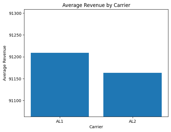
You don’t have to use altair for visualization, you can take the underlying data and visualize it
however you like, with whatever Python libraries you’re comfortable with. You can even make the
figures super misleading, if that suits your fancy!
import matplotlib.pyplot as plt

plt.bar(summary.carriers.index, summary.carriers["avg_rev"])
plt.xlabel("Carrier")
plt.ylabel("Average Revenue")
plt.title("Average Revenue by Carrier")
plt.ylim(summary.carriers["avg_rev"].min() - 100, summary.carriers["avg_rev"].max() + 100)
plt.show()
Bookings by Timeframe
summary.fig_bookings_by_timeframe()
If use the by_carrier argument to get the details for only a single carrier, PassengerSim will
automatically enhance the detail of the figure to drill down into passenger segments.
summary.fig_bookings_by_timeframe(by_carrier="AL1")
We can further drill down by fare classes. This will preserve the passenger segmentation, not as the bar colors but in seperate facet panels.
summary.fig_bookings_by_timeframe(by_carrier="AL1", by_class=True)
Underneath these figures is a segmentation by timeframe dataframe, which has data we can slice and dice in different ways.
summary.segmentation_by_timeframe
| metric | bookings | revenue | |||||
|---|---|---|---|---|---|---|---|
| segment | business | leisure | business | leisure | |||
| trial | carrier | booking_class | days_prior | ||||
| 0 | AL1 | Y0 | 1 | 2.325714 | 0.002857 | 1347.714286 | 1.428571 |
| 3 | 9.542857 | 0.025714 | 5595.285714 | 13.571429 | |||
| 5 | 4.577143 | 0.020000 | 2653.142857 | 10.714286 | |||
| 7 | 4.251429 | 0.002857 | 2493.428571 | 1.428571 | |||
| 10 | 6.722857 | 0.005714 | 3969.142857 | 2.857143 | |||
| ... | ... | ... | ... | ... | ... | ... | ... |
| 1 | NONE | XX | 35 | NaN | 1.488571 | NaN | NaN |
| 42 | NaN | 1.997143 | NaN | NaN | |||
| 49 | NaN | 1.577143 | NaN | NaN | |||
| 56 | NaN | 1.225714 | NaN | NaN | |||
| 63 | NaN | 2.385714 | NaN | NaN | |||
336 rows × 4 columns
Bid Prices
We also have a variety of bid price data that is tracked automatically, and which we can examine. The bid price history shows how the average bid prices evolve over time.
summary.fig_bid_price_history()
There are some technical oddities in the average bid prices. Most notably,
in the absence of overbooking the bid price isn’t defined for flights
that are sold out. The history visualized here uses a placeholder value for
those sold out flights: the bid price of the last seat, the moment before it was sold.
To show only the average bid prices for legs where there is some capacity
remaining, we can specify cap="some", and we will get a picture that
looks very similar, until the final few days prior to departure.
summary.fig_bid_price_history(cap="some")
Other Included Data
There is quite a variety of data in the summary object. You can see what’s available
as a list in the repr that displays for the summary.
summary
<passengersim.summaries.SimulationTables created on 2026-06-12>
 * bid_price_history (256 row DataFrame)
 * cabins (5600 row DataFrame)
 * carriers (2 row DataFrame)
 * carrier_history (NoneType)
 * carrier_history2 (1400 row DataFrame)
 * forecast_accuracy (NoneType)
 * cp_segmentation (12 row DataFrame)
 * demand_to_come_summary (34 row DataFrame)
 * demand_to_come (NoneType)
 * demands (6 row DataFrame)
 * demand_history (NoneType)
 * displacement_history (68 row DataFrame)
 * fare_class_mix (12 row DataFrame)
 * path_forecasts (NoneType)
 * leg_forecasts (NoneType)
 * edgar (NoneType)
 * legbuckets (48 row DataFrame)
 * legs (8 row DataFrame)
 * leg_detail (NoneType)
 * local_and_flow_yields (NoneType)
 * pathclasses (72 row DataFrame)
 * path_legs (16 row DataFrame)
 * paths (12 row DataFrame)
 * segmentation_by_timeframe (336 row DataFrame)
 * segmentation_detail (NoneType)
<*>
There are numerous data tables that have no canned visualizations attached to them, but that should not limit you to want you can look at in the results. Just as you can roll your own visualizations to replace existing ones, you can also do all kinds of novel analysis with the data that’s provided.
For example, let’s look at the data in the pathclasses table.
summary.pathclasses
| carrier | orig | dest | gt_revenue | gt_revenue_by_segment_business | gt_revenue_by_segment_leisure | gt_sold | gt_sold_by_segment_business | gt_sold_by_segment_leisure | gt_sold_priceable | ||
|---|---|---|---|---|---|---|---|---|---|---|---|
| path_id | booking_class | ||||||||||
| 1 | Y0 | AL1 | BOS | ORD | 667600.0 | 667200.0 | 400.0 | 1669 | 1668.0 | 1.0 | 81 |
| Y1 | AL1 | BOS | ORD | 2004600.0 | 1978500.0 | 26100.0 | 6682 | 6595.0 | 87.0 | 1809 | |
| Y2 | AL1 | BOS | ORD | 686600.0 | 605200.0 | 81400.0 | 3433 | 3026.0 | 407.0 | 1076 | |
| Y3 | AL1 | BOS | ORD | 154350.0 | 23550.0 | 130800.0 | 1029 | 157.0 | 872.0 | 751 | |
| Y4 | AL1 | BOS | ORD | 1006750.0 | 23750.0 | 983000.0 | 8054 | 190.0 | 7864.0 | 1313 | |
| ... | ... | ... | ... | ... | ... | ... | ... | ... | ... | ... | ... |
| 12 | Y1 | AL2 | BOS | LAX | 2738750.0 | 2671875.0 | 66875.0 | 4382 | 4275.0 | 107.0 | 1222 |
| Y2 | AL2 | BOS | LAX | 1767600.0 | 1561950.0 | 205650.0 | 3928 | 3471.0 | 457.0 | 1567 | |
| Y3 | AL2 | BOS | LAX | 631150.0 | 168025.0 | 463125.0 | 1942 | 517.0 | 1425.0 | 1614 | |
| Y4 | AL2 | BOS | LAX | 3199750.0 | 147500.0 | 3052250.0 | 12799 | 590.0 | 12209.0 | 4637 | |
| Y5 | AL2 | BOS | LAX | 818200.0 | 0.0 | 818200.0 | 4091 | 0.0 | 4091.0 | 4091 |
72 rows × 10 columns
All the columns prefixed by gt_ represent “grand total” values across all simulation samples (after the burn). You can easily
convert those columns to averages by dividing by the number of samples in the data.
pc = summary.pathclasses.filter(regex="^gt_")
pc.columns = pc.columns.str.removeprefix("gt_")
pc /= summary.n_total_samples
pc = summary.pathclasses.join(pc.add_prefix("average_"))
pc
| carrier | orig | dest | gt_revenue | gt_revenue_by_segment_business | gt_revenue_by_segment_leisure | gt_sold | gt_sold_by_segment_business | gt_sold_by_segment_leisure | gt_sold_priceable | average_revenue | average_revenue_by_segment_business | average_revenue_by_segment_leisure | average_sold | average_sold_by_segment_business | average_sold_by_segment_leisure | average_sold_priceable | ||
|---|---|---|---|---|---|---|---|---|---|---|---|---|---|---|---|---|---|---|
| path_id | booking_class | |||||||||||||||||
| 1 | Y0 | AL1 | BOS | ORD | 667600.0 | 667200.0 | 400.0 | 1669 | 1668.0 | 1.0 | 81 | 953.714286 | 953.142857 | 0.571429 | 2.384286 | 2.382857 | 0.001429 | 0.115714 |
| Y1 | AL1 | BOS | ORD | 2004600.0 | 1978500.0 | 26100.0 | 6682 | 6595.0 | 87.0 | 1809 | 2863.714286 | 2826.428571 | 37.285714 | 9.545714 | 9.421429 | 0.124286 | 2.584286 | |
| Y2 | AL1 | BOS | ORD | 686600.0 | 605200.0 | 81400.0 | 3433 | 3026.0 | 407.0 | 1076 | 980.857143 | 864.571429 | 116.285714 | 4.904286 | 4.322857 | 0.581429 | 1.537143 | |
| Y3 | AL1 | BOS | ORD | 154350.0 | 23550.0 | 130800.0 | 1029 | 157.0 | 872.0 | 751 | 220.500000 | 33.642857 | 186.857143 | 1.470000 | 0.224286 | 1.245714 | 1.072857 | |
| Y4 | AL1 | BOS | ORD | 1006750.0 | 23750.0 | 983000.0 | 8054 | 190.0 | 7864.0 | 1313 | 1438.214286 | 33.928571 | 1404.285714 | 11.505714 | 0.271429 | 11.234286 | 1.875714 | |
| ... | ... | ... | ... | ... | ... | ... | ... | ... | ... | ... | ... | ... | ... | ... | ... | ... | ... | ... |
| 12 | Y1 | AL2 | BOS | LAX | 2738750.0 | 2671875.0 | 66875.0 | 4382 | 4275.0 | 107.0 | 1222 | 3912.500000 | 3816.964286 | 95.535714 | 6.260000 | 6.107143 | 0.152857 | 1.745714 |
| Y2 | AL2 | BOS | LAX | 1767600.0 | 1561950.0 | 205650.0 | 3928 | 3471.0 | 457.0 | 1567 | 2525.142857 | 2231.357143 | 293.785714 | 5.611429 | 4.958571 | 0.652857 | 2.238571 | |
| Y3 | AL2 | BOS | LAX | 631150.0 | 168025.0 | 463125.0 | 1942 | 517.0 | 1425.0 | 1614 | 901.642857 | 240.035714 | 661.607143 | 2.774286 | 0.738571 | 2.035714 | 2.305714 | |
| Y4 | AL2 | BOS | LAX | 3199750.0 | 147500.0 | 3052250.0 | 12799 | 590.0 | 12209.0 | 4637 | 4571.071429 | 210.714286 | 4360.357143 | 18.284286 | 0.842857 | 17.441429 | 6.624286 | |
| Y5 | AL2 | BOS | LAX | 818200.0 | 0.0 | 818200.0 | 4091 | 0.0 | 4091.0 | 4091 | 1168.857143 | 0.000000 | 1168.857143 | 5.844286 | 0.000000 | 5.844286 | 5.844286 |
72 rows × 17 columns
df = (
    pc.query("carrier == 'AL1'")
    .rename(columns={"gt_revenue_by_segment_business": "Business", "gt_revenue_by_segment_leisure": "Leisure"})
    .reset_index()
    .melt(
        id_vars=["path_id", "booking_class"],
        value_vars=["Business", "Leisure"],
        var_name="segment",
        value_name="revenue",
    )
)

alt.Chart(df).mark_bar().encode(
    y="booking_class",
    x="revenue",
    color="segment",
    tooltip=["booking_class", "segment", "revenue"],
).facet(row="path_id")
Collecting Other Data with Callbacks
PassengerSim includes a variety of optimized data collection processes that run automatically during a simulation, but these pre-selected data may not be sufficient for every analysis. To supplement this, users can choose to additionally collect any other data while running a simulation. This is done by writing a “callback” function. Such a function is invoked regularly while the simulation is running, and can inspect and store almost anything from the Simulation object.
The primary thing to keep in mind about callbacks is that they are going to run during your simulation, so you have to set them up before running the simulation. You cannot do anything to change the callbacks once the simulation is finished any you have summary result object.
So, to demo the callbacks, we’ll create a new simulation but not run it (yet).
sim = pax.Simulation(cfg)
Types of Callback Functions
To collect data, we can write a function that will interrogate the simulation and grab whatever info we are looking for. There are three different points where we can attach data collection callback functions:
begin_sample, which will trigger data collection at the beginning of each sample, after the RM systems for each carrier are initialized (e.g. with forecasts, etc) but before any customers can arrive.end_sample, which will trigger data collection at the end of each sample, after customers have arrive and all bookings have be finalized.daily, which will trigger data collection once per day during every sample, just after any DCP or daily RM system updates are run.
The first two callbacks (begin and end sample) are written as a function that accepts one argument
(the Simulation object), and either returns nothing (to ignore that event)
or returns a dictionary of values to store, where the keys are all strings
naming what’s being stored and the values can be whatever is of interest.
This can be a simple numeric value (i.e., a scalar), or a tuple, an array,
a nested dictionary, or any other pickle-able
Python object.
We can attach each callback to the Simulation by using a Python decorator.
Example Callback Functions
For example, here we create a callback to collect carrier revenue at the end of every sample. Note that we skip the burn period by returning nothing for those samples; this is not required by the callback algorithm but is good practice for analysis.
@sim.end_sample_callback
def collect_carrier_revenue(sim: pax.Simulation) -> dict | None:
    if sim.eng.sample < sim.eng.burn_samples:
        return
    return {c.name: c.revenue for c in sim.eng.carriers}
The daily callback operates similarly, except it accepts a second argument that gives the number of days prior to departure for this day. You don’t need to use the second argument in the callback function, but you need to including in the function signature (and you can use it if desired, e.g. to collect data only at DCPs instead of every day). In the example here, we collect daily carrier revenue, but only every 7th sample, which is a good way to reduce the overhead from collecting detailed data.
@sim.daily_callback
def collect_carrier_revenue_detail(sim: pax.Simulation, days_prior: int) -> dict | None:
    if sim.eng.sample < sim.eng.burn_samples:
        return
    if sim.eng.sample % 7 == 0:
        return {c.name: c.revenue for c in sim.eng.carriers}
Multiple callbacks of the same kind can be attached (i.e. there can be two end_sample callbacks). The only limitation is that the named values in the return values of each callback function must be unique, or else they will overwrite one another.
For example, suppose we also want to count for each carrier the number of passengers departing each airport on each sample day. The previous end sample callback stored revenue values in a dictionary keyed by carrier name, so if we don’t want to overwrite that, we need to use a different key. One way to avoid that is to just nest the output of the callback function in another dictionary with a unique top level key.
from collections import defaultdict


@sim.end_sample_callback
def collect_passenger_counts(sim: pax.Simulation) -> dict | None:
    if sim.eng.sample < sim.eng.burn_samples:
        return
    paxcount = defaultdict(lambda: defaultdict(int))
    for leg in sim.eng.legs:
        paxcount[leg.carrier.name][leg.orig] += leg.sold
    # convert defaultdict to a regular dict, not necessary but pickles smaller
    paxcount = {carrier: dict(airports) for carrier, airports in paxcount.items()}
    return {"psgr_by_airport": paxcount}
One of the nifty features of callbacks is that they can access anything available in the simulation, not just sales and revenue data from carriers. For example, we can inspect demand objects directly, and see how many potential passengers were simulated so far, and how many didn’t make a booking on any airlines (i.e. the “no-go” customers).
@sim.daily_callback
def count_nogo(sim: pax.Simulation, days_prior: int) -> dict | None:
    if sim.eng.sample < sim.eng.burn_samples:
        return
    if sim.eng.sample % 7 == 0:
        return
    if days_prior > 0 and days_prior not in sim.config.dcps:
        # Only count "nogo" (unsold) demand at DCPs, and at departure (days_prior == 0)
        return
    nogo_count = defaultdict(lambda: defaultdict(lambda: defaultdict(int)))
    for dmd in sim.eng.demands:
        nogo_count[dmd.orig][dmd.dest][dmd.segment] += dmd.unsold
    # convert defaultdict to a regular dict, not necessary but pickles smaller
    nogo_count = {orig: {dest: dict(seg) for dest, seg in dests.items()} for orig, dests in nogo_count.items()}
    return {"nogo": nogo_count}
Re-using Callback Functions
Attaching via the decorators is a convenient way to add callbacks to a single simulation. The decorators connect the callback function to the simulation, but do not otherwise modify the function itself. It is easy to define callback functions in a seperate module or to re-use callback functions for multiple simulations, by using the decorator as a regular function. For example, we can create a second simulation object, and attach the same callback functions like this:
duplicate_sim = pax.Simulation(cfg)
duplicate_sim.end_sample_callback(collect_carrier_revenue)
duplicate_sim.daily_callback(collect_carrier_revenue_detail);
In this example, the duplicate_sim is running the same config as the original, but this would work with a modified config or even a completely different network.
Once we have attached all desired callbacks to the simulation we want to run, we can run it as normal.
summary = sim.run()
Task Completed after 9.45 seconds
All the usual summary data remains available for review and analysis.
summary.fig_carrier_revenues()
Callback Data
In addition to the usual suspects, the summary object includes the collected callback data from our callback functions.
summary.callback_data
<passengersim.callbacks.base.CallbackData from daily, end_sample>
Because we connected a “daily” callback, the data we collected is available under the
callback_data.daily accessor.
summary.callback_data.daily[:5]
[{'trial': 0,
  'sample': 50,
  'days_prior': 63,
  'nogo': {'BOS': {'ORD': {'business': 0, 'leisure': 0},
    'LAX': {'business': 0, 'leisure': 0}},
   'ORD': {'LAX': {'business': 0, 'leisure': 0}}}},
 {'trial': 0,
  'sample': 50,
  'days_prior': 56,
  'nogo': {'BOS': {'ORD': {'business': 0, 'leisure': 0},
    'LAX': {'business': 0, 'leisure': 0}},
   'ORD': {'LAX': {'business': 0, 'leisure': 0}}}},
 {'trial': 0,
  'sample': 50,
  'days_prior': 49,
  'nogo': {'BOS': {'ORD': {'business': 0, 'leisure': 0},
    'LAX': {'business': 0, 'leisure': 0}},
   'ORD': {'LAX': {'business': 0, 'leisure': 0}}}},
 {'trial': 0,
  'sample': 50,
  'days_prior': 42,
  'nogo': {'BOS': {'ORD': {'business': 0, 'leisure': 0},
    'LAX': {'business': 0, 'leisure': 0}},
   'ORD': {'LAX': {'business': 0, 'leisure': 0}}}},
 {'trial': 0,
  'sample': 50,
  'days_prior': 35,
  'nogo': {'BOS': {'ORD': {'business': 0, 'leisure': 0},
    'LAX': {'business': 0, 'leisure': 0}},
   'ORD': {'LAX': {'business': 0, 'leisure': 0}}}}]
As you might expect, the “begin_sample” or “end_sample”
callbacks are available under callback_data.begin_sample or callback_data.end_sample,
respectively.
summary.callback_data.end_sample[:3]
[{'trial': 0,
  'sample': 50,
  'AL1': 80300.0,
  'AL2': 83425.0,
  'psgr_by_airport': {'AL1': {'BOS': 158.0, 'ORD': 180.0},
   'AL2': {'BOS': 155.0, 'ORD': 195.0}}},
 {'trial': 0,
  'sample': 51,
  'psgr_by_airport': {'AL1': {'BOS': 159.0, 'ORD': 220.0},
   'AL2': {'BOS': 150.0, 'ORD': 193.0}},
  'AL1': 86100.0,
  'AL2': 75200.0},
 {'trial': 0,
  'sample': 52,
  'AL1': 91725.0,
  'AL2': 96200.0,
  'psgr_by_airport': {'AL1': {'BOS': 190.0, 'ORD': 229.0},
   'AL2': {'BOS': 194.0, 'ORD': 223.0}}}]
The callback data can include pretty much anything, so it is stored in a
very flexible (but inefficient) format: a list of dict’s. If the content
of the dicts is fairly simple (numbers, tuples, lists, or nested dictionaries thereof),
it can be converted into a pandas DataFrame using the to_dataframe method
on the callback_data attribute. This may make subsequent analysis easier.
summary.callback_data.to_dataframe("daily")
| trial | sample | days_prior | nogo.BOS.ORD.business | nogo.BOS.ORD.leisure | nogo.BOS.LAX.business | nogo.BOS.LAX.leisure | nogo.ORD.LAX.business | nogo.ORD.LAX.leisure | AL1 | AL2 | |
|---|---|---|---|---|---|---|---|---|---|---|---|
| 0 | 0 | 50 | 63 | 0.0 | 0.0 | 0.0 | 0.0 | 0.0 | 0.0 | NaN | NaN |
| 1 | 0 | 50 | 56 | 0.0 | 0.0 | 0.0 | 0.0 | 0.0 | 0.0 | NaN | NaN |
| 2 | 0 | 50 | 49 | 0.0 | 0.0 | 0.0 | 0.0 | 0.0 | 0.0 | NaN | NaN |
| 3 | 0 | 50 | 42 | 0.0 | 0.0 | 0.0 | 0.0 | 0.0 | 0.0 | NaN | NaN |
| 4 | 0 | 50 | 35 | 0.0 | 0.0 | 0.0 | 0.0 | 0.0 | 0.0 | NaN | NaN |
| ... | ... | ... | ... | ... | ... | ... | ... | ... | ... | ... | ... |
| 16595 | 1 | 399 | 4 | NaN | NaN | NaN | NaN | NaN | NaN | 75075.0 | 77475.0 |
| 16596 | 1 | 399 | 3 | NaN | NaN | NaN | NaN | NaN | NaN | 79975.0 | 79275.0 |
| 16597 | 1 | 399 | 2 | NaN | NaN | NaN | NaN | NaN | NaN | 88000.0 | 82950.0 |
| 16598 | 1 | 399 | 1 | NaN | NaN | NaN | NaN | NaN | NaN | 91725.0 | 85250.0 |
| 16599 | 1 | 399 | 0 | NaN | NaN | NaN | NaN | NaN | NaN | 95250.0 | 86050.0 |
16600 rows × 11 columns
summary.callback_data.to_dataframe("end_sample")
| trial | sample | AL1 | AL2 | psgr_by_airport.AL1.BOS | psgr_by_airport.AL1.ORD | psgr_by_airport.AL2.BOS | psgr_by_airport.AL2.ORD | |
|---|---|---|---|---|---|---|---|---|
| 0 | 0 | 50 | 80300.0 | 83425.0 | 158.0 | 180.0 | 155.0 | 195.0 |
| 1 | 0 | 51 | 86100.0 | 75200.0 | 159.0 | 220.0 | 150.0 | 193.0 |
| 2 | 0 | 52 | 91725.0 | 96200.0 | 190.0 | 229.0 | 194.0 | 223.0 |
| 3 | 0 | 53 | 96100.0 | 92750.0 | 200.0 | 226.0 | 200.0 | 205.0 |
| 4 | 0 | 54 | 99675.0 | 99625.0 | 164.0 | 240.0 | 195.0 | 240.0 |
| ... | ... | ... | ... | ... | ... | ... | ... | ... |
| 695 | 1 | 395 | 84275.0 | 90900.0 | 168.0 | 221.0 | 172.0 | 219.0 |
| 696 | 1 | 396 | 88600.0 | 85125.0 | 196.0 | 190.0 | 180.0 | 181.0 |
| 697 | 1 | 397 | 100900.0 | 95600.0 | 196.0 | 238.0 | 197.0 | 229.0 |
| 698 | 1 | 398 | 88575.0 | 84325.0 | 198.0 | 185.0 | 191.0 | 169.0 |
| 699 | 1 | 399 | 95250.0 | 86050.0 | 132.0 | 215.0 | 130.0 | 192.0 |
700 rows × 8 columns
Users are free to process this callback data now however they like, with typical Python tools: analyze, visualize, interpret, etc.
# Visualize revenue difference between carriers across booking curve

import altair as alt

df = summary.callback_data.to_dataframe("daily").eval("DIFF = AL1 - AL2").query("sample < 100 and trial == 0")

alt.Chart(df).mark_line().encode(
    x=alt.X("days_prior", scale=alt.Scale(reverse=True)),
    y="DIFF",
    color="sample:N",
)
# Visualize "nogo" passengers over time, by market and segment

nogo = (
    summary.callback_data.to_dataframe("daily")
    .set_index(["days_prior", "sample"])
    .drop(columns=["trial", "AL1", "AL2"])
)
nogo.columns = pd.MultiIndex.from_tuples(nogo.columns.str.split(".").to_list())
nogo.columns.names = ["nogo", "orig", "dest", "segment"]
nogo = nogo.stack([1, 2, 3], future_stack=True).dropna().reset_index()

mean_nogo = nogo.groupby(["days_prior", "orig", "dest", "segment"]).nogo.mean().reset_index()
mean_nogo["market"] = mean_nogo.orig + "-" + mean_nogo.dest

alt.Chart(mean_nogo).mark_line().encode(
    x=alt.X("days_prior", scale=alt.Scale(reverse=True)),
    y="nogo",
    color="segment:N",
    strokeWidth="market:N",
    strokeDash="market:N",
)
Tracing
In addition to the completely flexible callback data storage system,
PassengerSim also includes the ability to “trace” certain details of the
simulation. Traces are more aggregate than other callbacks, as they will
follow the average values of various measures over many samples. Unlike
other aggregate measures, they allow for the selection of a limited number of
micro-level details, e.g. path forecasts for specific paths, or bid prices on
specific legs. This contrasts with the database functionality, which can
(relatively) efficiently store this information for all paths or legs.
Tracing allows the analyst to probe a simulation for details of interest
without becoming bogged down in the recording and storage of massive amounts
of data that really isn’t needed.
sim = pax.Simulation(cfg)
Forecast Tracing
The path forecast tracing capabilities allows us to record detailed data about a subset of Simulation path forecasts, so we can review them after the simulation. The tracing will summarize the average forecasts for the specific paths, but will not store the sample-by-sample forecast details, which would be an enormous amount of detail that will require large amounts of memory or disk storage and may not be sufficiently useful for analysis. A similar tracing tool is available for leg forecasts as well.
from passengersim.tracers.forecasts import (
    PathForecastTracer,
    fig_path_forecast_dashboard,
)

f_tracer = PathForecastTracer(path_ids=[1, 5, 9])
f_tracer.attach(sim)
Bid Price Tracing
Similarly, the bid price tracing feature allows us to record detailed data about a subset of Simulation bid prices. We can record bid prices by leg, path, or both if desired. Each tracer only attaches to the bid prices on a selected subset of individual legs, so as to not overwhelm the simulation with data.
from passengersim.tracers.bid_price import (
    LegBidPriceTracer,
    PathBidPriceTracer,
    fig_leg_bid_prices,
    fig_path_bid_prices,
)

bp_tracer = PathBidPriceTracer(path_ids=[1, 5, 9])
bp_tracer.attach(sim)

leg_bp_tracer = LegBidPriceTracer(leg_ids=[101, 111])
leg_bp_tracer.attach(sim)
Once the tracers have been attached, we run the simulation as normal. The attached tracers will automatically collect and aggregate the relevant data, and attach the tabulated results to the summary outputs.
summary = sim.run()
Task Completed after 11.57 seconds
All the usual summary data remains available for review and analysis.
summary.fig_carrier_revenues()
summary.fig_fare_class_mix()
Dashboards
In addition to the usual summary reports, the output summary also provides the data needed to power detailed dashboard visualizations for each of the traced paths or legs.
For the selected paths or legs, we can review a forecast dashboard that shows the forecast mean and std dev for each fare class from each DCP through departure, the mean forecast within each timeframe, as well as history data on yieldable and (if recorded separately) priceable sales, and average closure rates at each DCP. The displayed data in each dashboard is specific to the selected path or leg, but averaged across all relevant (non-burned) samples in the simulation.
fig_path_forecast_dashboard(summary, path_id=1)
fig_path_forecast_dashboard(summary, path_id=5)
fig_path_forecast_dashboard(summary, path_id=9)
The dashboards for bid price tracing are less busy than those for the forecasts, as the bid price
fig_path_bid_prices(summary)
fig_leg_bid_prices(summary)
Tracers in Callback Data
All the underlying data for these reports is stored in the summary’s callback_data attribute, if you want to access
it to parse or visualize it differently. The forecast tracers contain selected summary statistics by path or leg, days prior, and fare class. These statistics are aggregated across all relevant (i.e. non-burned) samples.
summary.callback_data.selected_path_forecasts
| mean_to_departure | stdev_to_departure | ... | history_sold_yieldable | history_closure | ||||||||||||||||||
|---|---|---|---|---|---|---|---|---|---|---|---|---|---|---|---|---|---|---|---|---|---|---|
| booking_class | Y0 | Y1 | Y2 | Y3 | Y4 | Y5 | Y0 | Y1 | Y2 | Y3 | ... | Y2 | Y3 | Y4 | Y5 | Y0 | Y1 | Y2 | Y3 | Y4 | Y5 | |
| path_id | days_prior | |||||||||||||||||||||
| 1 | 63 | 2.559180 | 10.061166 | 5.387678 | 1.837527 | 12.116845 | 6.457167 | 1.783795 | 4.285100 | 2.733197 | 1.660695 | ... | 0.323736 | 0.069670 | 2.393571 | 1.462912 | 0.000000 | 0.000000 | 0.000000 | 0.000000 | 0.000000 | 0.011429 |
| 56 | 2.421873 | 9.563914 | 5.063942 | 1.767857 | 9.723274 | 4.981590 | 1.724741 | 4.115693 | 2.631284 | 1.616743 | ... | 0.251429 | 0.061813 | 1.117527 | 0.626538 | 0.000000 | 0.000000 | 0.000000 | 0.000000 | 0.000000 | 0.028571 | |
| 49 | 2.303741 | 9.092155 | 4.812514 | 1.706043 | 8.605746 | 4.329498 | 1.662070 | 3.989028 | 2.586396 | 1.581816 | ... | 0.232253 | 0.040275 | 1.300110 | 0.797912 | 0.000000 | 0.000000 | 0.000000 | 0.000000 | 0.001429 | 0.050055 | |
| 42 | 2.224400 | 8.761991 | 4.580261 | 1.665769 | 7.304719 | 3.480202 | 1.630084 | 3.843912 | 2.517522 | 1.554698 | ... | 0.276044 | 0.050000 | 1.363846 | 0.750549 | 0.000000 | 0.000000 | 0.000000 | 0.001429 | 0.014286 | 0.094725 | |
| 35 | 2.133796 | 8.276056 | 4.304217 | 1.615654 | 5.925615 | 2.639771 | 1.600810 | 3.664363 | 2.417010 | 1.541537 | ... | 0.175220 | 0.026099 | 0.853626 | 0.522747 | 0.000000 | 0.000000 | 0.000000 | 0.001429 | 0.026923 | 0.126484 | |
| 31 | 2.069345 | 7.983639 | 4.128997 | 1.589555 | 5.042210 | 2.008268 | 1.600119 | 3.540281 | 2.348635 | 1.522014 | ... | 0.121264 | 0.025330 | 0.549560 | 0.330934 | 0.000000 | 0.000000 | 0.000000 | 0.005495 | 0.040275 | 0.137692 | |
| 28 | 2.029565 | 7.813199 | 4.007733 | 1.563105 | 4.459351 | 1.592600 | 1.604541 | 3.478925 | 2.288687 | 1.499428 | ... | 0.145879 | 0.050220 | 1.145769 | 0.659890 | 0.000000 | 0.000000 | 0.000000 | 0.022637 | 0.068846 | 0.170385 | |
| 24 | 1.980169 | 7.573804 | 3.861854 | 1.491848 | 3.233781 | 0.766361 | 1.584625 | 3.421044 | 2.244300 | 1.365275 | ... | 0.164945 | 0.065000 | 1.052473 | 0.579451 | 0.000000 | 0.000000 | 0.004286 | 0.044396 | 0.116209 | 0.203297 | |
| 21 | 1.919620 | 7.268309 | 3.695538 | 1.415540 | 2.046767 | 0.000000 | 1.561706 | 3.313309 | 2.169436 | 1.265751 | ... | 0.235440 | 0.082473 | 0.933022 | 0.000000 | 0.000000 | 0.000000 | 0.019670 | 0.070659 | 0.149286 | 1.000000 | |
| 17 | 1.832257 | 6.912540 | 3.448764 | 1.308515 | 0.927720 | 0.000000 | 1.533422 | 3.200638 | 2.042170 | 1.160598 | ... | 0.307088 | 0.074451 | 0.743736 | 0.000000 | 0.000000 | 0.001099 | 0.033736 | 0.105879 | 0.174835 | 1.000000 | |
| 14 | 1.741818 | 6.424103 | 3.121025 | 1.201217 | 0.000000 | 0.000000 | 1.485598 | 3.066562 | 1.872077 | 1.057076 | ... | 0.649341 | 0.561209 | 0.000000 | 0.000000 | 0.000000 | 0.005385 | 0.062967 | 0.151374 | 1.000000 | 1.000000 | |
| 10 | 1.520774 | 5.412324 | 2.420786 | 0.506886 | 0.000000 | 0.000000 | 1.363206 | 2.688997 | 1.575241 | 0.629111 | ... | 0.666923 | 0.378462 | 0.000000 | 0.000000 | 0.005385 | 0.024341 | 0.118022 | 0.189341 | 1.000000 | 1.000000 | |
| 7 | 1.218199 | 4.265386 | 1.651783 | 0.000000 | 0.000000 | 0.000000 | 1.161100 | 2.216533 | 1.204525 | 0.000000 | ... | 0.599341 | 0.000000 | 0.000000 | 0.000000 | 0.009396 | 0.049670 | 0.145165 | 1.000000 | 1.000000 | 1.000000 | |
| 5 | 1.032603 | 3.494357 | 0.921951 | 0.000000 | 0.000000 | 0.000000 | 1.050092 | 1.946856 | 0.856543 | 0.000000 | ... | 0.747637 | 0.000000 | 0.000000 | 0.000000 | 0.021593 | 0.066154 | 0.166154 | 1.000000 | 1.000000 | 1.000000 | |
| 3 | 0.839314 | 2.707654 | 0.000000 | 0.000000 | 0.000000 | 0.000000 | 0.912073 | 1.631885 | 0.000000 | 0.000000 | ... | 0.000000 | 0.000000 | 0.000000 | 0.000000 | 0.125220 | 0.140934 | 1.000000 | 1.000000 | 1.000000 | 1.000000 | |
| 1 | 0.216548 | 0.708058 | 0.000000 | 0.000000 | 0.000000 | 0.000000 | 0.373929 | 0.768418 | 0.000000 | 0.000000 | ... | 0.000000 | 0.000000 | 0.000000 | 0.000000 | 0.212747 | 0.217033 | 1.000000 | 1.000000 | 1.000000 | 1.000000 | |
| 5 | 63 | 15.186842 | 11.386570 | 4.391357 | 4.003982 | 25.469384 | 7.659940 | 6.018443 | 4.568701 | 2.525438 | 3.951949 | ... | 0.206374 | 0.052473 | 5.117308 | 0.829176 | 0.000000 | 0.000000 | 0.000000 | 0.000000 | 0.002692 | 0.630549 |
| 56 | 14.262996 | 10.722614 | 4.184983 | 3.951509 | 20.347845 | 6.039138 | 5.698689 | 4.372888 | 2.462001 | 3.941090 | ... | 0.203736 | 0.039396 | 2.469560 | 0.417912 | 0.000000 | 0.000000 | 0.000000 | 0.000000 | 0.023022 | 0.579176 | |
| 49 | 13.486732 | 10.175636 | 3.981247 | 3.912114 | 17.841954 | 5.021001 | 5.441160 | 4.220048 | 2.381499 | 3.911447 | ... | 0.152253 | 0.071703 | 2.685714 | 0.469615 | 0.000000 | 0.000000 | 0.000000 | 0.000000 | 0.069451 | 0.555714 | |
| 42 | 12.931568 | 9.772614 | 3.828994 | 3.840410 | 15.020926 | 3.929829 | 5.244726 | 4.074104 | 2.344333 | 3.816578 | ... | 0.175989 | 0.167637 | 2.722912 | 0.525714 | 0.000000 | 0.000000 | 0.000000 | 0.001374 | 0.137582 | 0.528516 | |
| 35 | 12.171293 | 9.256845 | 3.653005 | 3.670536 | 11.998233 | 2.741738 | 5.006553 | 3.911499 | 2.261916 | 3.545094 | ... | 0.110110 | 0.145110 | 1.679341 | 0.316154 | 0.000000 | 0.000000 | 0.000000 | 0.001374 | 0.180275 | 0.493022 | |
| 31 | 11.755579 | 8.949482 | 3.542895 | 3.525057 | 9.998358 | 2.009841 | 4.876112 | 3.818044 | 2.209195 | 3.313745 | ... | 0.083956 | 0.141868 | 1.107308 | 0.177967 | 0.000000 | 0.000000 | 0.000000 | 0.005495 | 0.202198 | 0.473187 | |
| 28 | 11.458875 | 8.752504 | 3.458939 | 3.380585 | 8.612545 | 1.565941 | 4.774925 | 3.730515 | 2.167324 | 3.082741 | ... | 0.107308 | 0.328516 | 2.000769 | 0.392582 | 0.000000 | 0.000000 | 0.000000 | 0.015330 | 0.246703 | 0.468626 | |
| 24 | 10.996622 | 8.446735 | 3.351631 | 3.040136 | 6.055702 | 0.743247 | 4.588117 | 3.649565 | 2.108616 | 2.562244 | ... | 0.148571 | 0.365824 | 1.835165 | 0.348516 | 0.000000 | 0.000000 | 0.004176 | 0.068571 | 0.303901 | 0.475220 | |
| 21 | 10.552447 | 8.125306 | 3.199659 | 2.611299 | 3.553112 | 0.000000 | 4.455131 | 3.529741 | 2.012652 | 2.033733 | ... | 0.213187 | 0.278901 | 1.321429 | 0.000000 | 0.000000 | 0.000000 | 0.013956 | 0.127088 | 0.336429 | 1.000000 | |
| 17 | 9.978546 | 7.702394 | 2.978045 | 2.235239 | 1.615636 | 0.000000 | 4.238593 | 3.390274 | 1.877330 | 1.584000 | ... | 0.233132 | 0.199780 | 1.075824 | 0.000000 | 0.000000 | 0.000000 | 0.043516 | 0.190440 | 0.355110 | 1.000000 | |
| 14 | 9.253765 | 7.164647 | 2.722571 | 1.922805 | 0.000000 | 0.000000 | 4.025514 | 3.224215 | 1.707656 | 1.307292 | ... | 0.516538 | 0.857527 | 0.000000 | 0.000000 | 0.000000 | 0.018462 | 0.098736 | 0.240385 | 1.000000 | 1.000000 | |
| 10 | 7.777337 | 6.047116 | 2.127087 | 0.775043 | 0.000000 | 0.000000 | 3.587533 | 2.805084 | 1.395882 | 0.750757 | ... | 0.427692 | 0.505055 | 0.000000 | 0.000000 | 0.002857 | 0.051154 | 0.182253 | 0.294011 | 1.000000 | 1.000000 | |
| 7 | 5.969240 | 4.773215 | 1.568735 | 0.000000 | 0.000000 | 0.000000 | 2.893360 | 2.355585 | 1.137855 | 0.000000 | ... | 0.474286 | 0.000000 | 0.000000 | 0.000000 | 0.009835 | 0.101538 | 0.230165 | 1.000000 | 1.000000 | 1.000000 | |
| 5 | 4.768420 | 3.805097 | 0.908356 | 0.000000 | 0.000000 | 0.000000 | 2.489004 | 1.951915 | 0.848609 | 0.000000 | ... | 0.654176 | 0.000000 | 0.000000 | 0.000000 | 0.028242 | 0.136044 | 0.234341 | 1.000000 | 1.000000 | 1.000000 | |
| 3 | 3.494903 | 2.927920 | 0.000000 | 0.000000 | 0.000000 | 0.000000 | 2.003097 | 1.701909 | 0.000000 | 0.000000 | ... | 0.000000 | 0.000000 | 0.000000 | 0.000000 | 0.154066 | 0.231429 | 1.000000 | 1.000000 | 1.000000 | 1.000000 | |
| 1 | 0.849849 | 0.861825 | 0.000000 | 0.000000 | 0.000000 | 0.000000 | 0.761982 | 0.741407 | 0.000000 | 0.000000 | ... | 0.000000 | 0.000000 | 0.000000 | 0.000000 | 0.330879 | 0.377473 | 1.000000 | 1.000000 | 1.000000 | 1.000000 | |
| 9 | 63 | 11.103951 | 6.560624 | 5.882186 | 3.017021 | 19.626348 | 11.883501 | 4.516991 | 3.124037 | 2.848464 | 2.428953 | ... | 0.297143 | 0.081264 | 3.894286 | 2.685055 | 0.000000 | 0.000000 | 0.000000 | 0.000000 | 0.000000 | 0.267912 |
| 56 | 10.464446 | 6.218261 | 5.585043 | 2.935757 | 15.732062 | 8.570873 | 4.322308 | 2.962983 | 2.743329 | 2.393684 | ... | 0.233297 | 0.045495 | 1.965549 | 0.965055 | 0.000000 | 0.000000 | 0.000000 | 0.000000 | 0.000000 | 0.352198 | |
| 49 | 10.003182 | 5.901558 | 5.351746 | 2.890262 | 13.766513 | 7.127339 | 4.189858 | 2.868320 | 2.658696 | 2.391530 | ... | 0.241209 | 0.049835 | 2.264341 | 1.075604 | 0.000000 | 0.000000 | 0.000000 | 0.000000 | 0.004286 | 0.393626 | |
| 42 | 9.553182 | 5.662602 | 5.110537 | 2.840427 | 11.497186 | 5.440017 | 4.032858 | 2.812264 | 2.582201 | 2.396957 | ... | 0.276538 | 0.067198 | 2.144231 | 0.880714 | 0.000000 | 0.000000 | 0.000000 | 0.000000 | 0.021154 | 0.432747 | |
| 35 | 9.026644 | 5.351338 | 4.833999 | 2.773229 | 9.314831 | 3.932039 | 3.847413 | 2.723374 | 2.468119 | 2.359324 | ... | 0.161703 | 0.071648 | 1.466264 | 0.545989 | 0.000000 | 0.000000 | 0.000000 | 0.000000 | 0.048077 | 0.437418 | |
| 31 | 8.687853 | 5.162107 | 4.672296 | 2.701581 | 7.782365 | 2.949924 | 3.781800 | 2.623482 | 2.402699 | 2.253501 | ... | 0.105495 | 0.050165 | 0.941758 | 0.341374 | 0.000000 | 0.000000 | 0.000000 | 0.000000 | 0.070440 | 0.415385 | |
| 28 | 8.494116 | 5.039525 | 4.566801 | 2.651416 | 6.768748 | 2.299707 | 3.723070 | 2.589168 | 2.366422 | 2.191749 | ... | 0.170440 | 0.150879 | 1.730275 | 0.669505 | 0.000000 | 0.000000 | 0.000000 | 0.007033 | 0.114615 | 0.407967 | |
| 24 | 8.206094 | 4.865788 | 4.396362 | 2.489822 | 4.843717 | 1.155165 | 3.595618 | 2.536165 | 2.293058 | 1.935953 | ... | 0.192637 | 0.217473 | 1.534560 | 0.638626 | 0.000000 | 0.000000 | 0.000000 | 0.027033 | 0.198571 | 0.440879 | |
| 21 | 7.887853 | 4.709415 | 4.203724 | 2.247742 | 2.997028 | 0.000000 | 3.483025 | 2.444788 | 2.207301 | 1.604009 | ... | 0.258352 | 0.212473 | 1.223407 | 0.000000 | 0.000000 | 0.000000 | 0.001319 | 0.059890 | 0.242527 | 1.000000 | |
| 17 | 7.436918 | 4.454085 | 3.944684 | 2.002968 | 1.409023 | 0.000000 | 3.330547 | 2.349042 | 2.073989 | 1.359847 | ... | 0.311044 | 0.160714 | 1.020714 | 0.000000 | 0.000000 | 0.000000 | 0.009890 | 0.109670 | 0.279890 | 1.000000 | |
| 14 | 6.869995 | 4.130019 | 3.629059 | 1.793501 | 0.000000 | 0.000000 | 3.135965 | 2.229251 | 1.929521 | 1.199806 | ... | 0.751538 | 0.820934 | 0.000000 | 0.000000 | 0.000000 | 0.000000 | 0.025440 | 0.185714 | 1.000000 | 1.000000 | |
| 10 | 5.831479 | 3.515294 | 2.855408 | 0.783527 | 0.000000 | 0.000000 | 2.796127 | 2.029926 | 1.682518 | 0.755690 | ... | 0.849011 | 0.546703 | 0.000000 | 0.000000 | 0.000000 | 0.002747 | 0.080604 | 0.265110 | 1.000000 | 1.000000 | |
| 7 | 4.443512 | 2.779744 | 1.932507 | 0.000000 | 0.000000 | 0.000000 | 2.278990 | 1.683320 | 1.292947 | 0.000000 | ... | 0.726648 | 0.000000 | 0.000000 | 0.000000 | 0.000000 | 0.015385 | 0.132857 | 1.000000 | 1.000000 | 1.000000 | |
| 5 | 3.634776 | 2.361663 | 1.073783 | 0.000000 | 0.000000 | 0.000000 | 1.989964 | 1.501351 | 0.916633 | 0.000000 | ... | 0.870934 | 0.000000 | 0.000000 | 0.000000 | 0.002747 | 0.033626 | 0.172473 | 1.000000 | 1.000000 | 1.000000 | |
| 3 | 2.776804 | 1.845339 | 0.000000 | 0.000000 | 0.000000 | 0.000000 | 1.661607 | 1.184247 | 0.000000 | 0.000000 | ... | 0.000000 | 0.000000 | 0.000000 | 0.000000 | 0.191154 | 0.191154 | 1.000000 | 1.000000 | 1.000000 | 1.000000 | |
| 1 | 0.705018 | 0.535657 | 0.000000 | 0.000000 | 0.000000 | 0.000000 | 0.638549 | 0.507425 | 0.000000 | 0.000000 | ... | 0.000000 | 0.000000 | 0.000000 | 0.000000 | 0.409341 | 0.413352 | 1.000000 | 1.000000 | 1.000000 | 1.000000 | |
48 rows × 36 columns
The bid prices data includes the mean and standard deviation of the leg or path bid price, by days prior.
summary.callback_data.leg_bid_prices
| leg_id | 101 | 111 | |
|---|---|---|---|
| statistic | days_prior | ||
| mean | 63 | 31.619009 | 138.467792 |
| 62 | 31.870381 | 138.442572 | |
| 61 | 31.845788 | 138.094838 | |
| 60 | 31.999171 | 137.646250 | |
| 59 | 32.593171 | 137.502162 | |
| ... | ... | ... | ... |
| std_dev | 4 | 116.045042 | 173.977634 |
| 3 | 112.005295 | 166.150435 | |
| 2 | 130.636388 | 185.540070 | |
| 1 | 154.677297 | 218.362993 | |
| 0 | 170.361355 | 240.804799 |
128 rows × 2 columns
Relationship to Callbacks
Unlike other callback data, the tracers are not stored by sample day, as that would generally create an overwhelming amount of data to store, and we are typically not interested in that much detail. If we are interested in grabbing and storing path forecast data for individual sample days, we can still do that with the regular callback interface.
sim1 = pax.Simulation(cfg)
@sim1.begin_sample_callback
def grab_forecasts(sim):
    if sim.eng.sample not in [300, 375]:
        return
    return {f"path-{p}": sim.eng.paths.select(path_id=p).get_forecast_data() for p in [1, 5, 9]}
summary1 = sim1.run()
Task Completed after 9.27 seconds
When run like this, we capture not the average path forecast over the simulation,
but rather the exact path forecast for the selected paths (1 and 9) at
sample days 300 and 375. The data is stored in the callback_data.begin_sample
attribute:
summary1.callback_data.begin_sample
[{'trial': 0,
  'sample': 300,
  'path-1': <passengersim_core.forecast_tools.ForecastData at 0x11dca03e0>,
  'path-5': <passengersim_core.forecast_tools.ForecastData at 0x11e38c740>,
  'path-9': <passengersim_core.forecast_tools.ForecastData at 0x11e38e000>},
 {'trial': 0,
  'sample': 375,
  'path-1': <passengersim_core.forecast_tools.ForecastData at 0x11e3ac0b0>,
  'path-5': <passengersim_core.forecast_tools.ForecastData at 0x11e3acbc0>,
  'path-9': <passengersim_core.forecast_tools.ForecastData at 0x11e3ae0f0>},
 {'trial': 1,
  'sample': 300,
  'path-1': <passengersim_core.forecast_tools.ForecastData at 0x11e3afbc0>,
  'path-5': <passengersim_core.forecast_tools.ForecastData at 0x11e3e8ef0>,
  'path-9': <passengersim_core.forecast_tools.ForecastData at 0x11dd7edb0>},
 {'trial': 1,
  'sample': 375,
  'path-1': <passengersim_core.forecast_tools.ForecastData at 0x11dd7dd90>,
  'path-5': <passengersim_core.forecast_tools.ForecastData at 0x11dd7c770>,
  'path-9': <passengersim_core.forecast_tools.ForecastData at 0x11dda6de0>}]
We can review the details of each specific forecast by accessing the dashboard visualization.
summary1.callback_data.begin_sample[0]["path-1"].dashboard()
We can also access individual sub-tables of forecast data as pandas DataFrames, to manipulate or visualize as we like.
summary1.callback_data.begin_sample[0]["path-1"].history_sold_yieldable
| booking_class | Y0 | Y1 | Y2 | Y3 | Y4 | Y5 |
|---|---|---|---|---|---|---|
| tf_index | ||||||
| 0 | 0.038462 | 0.500000 | 0.230769 | 0.076923 | 2.730769 | 1.307692 |
| 1 | 0.230769 | 0.423077 | 0.307692 | 0.038462 | 1.115385 | 0.423077 |
| 2 | 0.038462 | 0.692308 | 0.307692 | 0.038462 | 1.384615 | 0.923077 |
| 3 | 0.038462 | 0.846154 | 0.346154 | 0.038462 | 1.346154 | 0.692308 |
| 4 | 0.115385 | 0.461538 | 0.153846 | 0.038462 | 0.807692 | 0.500000 |
| 5 | 0.038462 | 0.192308 | 0.153846 | 0.000000 | 0.615385 | 0.115385 |
| 6 | 0.038462 | 0.153846 | 0.192308 | 0.076923 | 1.346154 | 0.769231 |
| 7 | 0.038462 | 0.384615 | 0.230769 | 0.000000 | 1.115385 | 0.538462 |
| 8 | 0.115385 | 0.230769 | 0.269231 | 0.038462 | 1.038462 | 0.000000 |
| 9 | 0.115385 | 0.500000 | 0.269231 | 0.076923 | 0.769231 | 0.000000 |
| 10 | 0.230769 | 1.269231 | 0.538462 | 0.615385 | 0.000000 | 0.000000 |
| 11 | 0.500000 | 1.153846 | 0.500000 | 0.423077 | 0.000000 | 0.000000 |
| 12 | 0.115385 | 1.038462 | 0.730769 | 0.000000 | 0.000000 | 0.000000 |
| 13 | 0.192308 | 0.923077 | 0.846154 | 0.000000 | 0.000000 | 0.000000 |
| 14 | 0.692308 | 2.538462 | 0.000000 | 0.000000 | 0.000000 | 0.000000 |
| 15 | 0.230769 | 0.538462 | 0.000000 | 0.000000 | 0.000000 | 0.000000 |
summary1.callback_data.begin_sample[0]["path-1"].mean_in_timeframe
| booking_class | Y0 | Y1 | Y2 | Y3 | Y4 | Y5 |
|---|---|---|---|---|---|---|
| tf_index | ||||||
| 0 | 0.038462 | 0.500000 | 0.230769 | 0.076923 | 2.730769 | 1.307692 |
| 1 | 0.230769 | 0.423077 | 0.307692 | 0.038462 | 1.115385 | 0.450537 |
| 2 | 0.038462 | 0.692308 | 0.307692 | 0.038462 | 1.384615 | 1.093785 |
| 3 | 0.038462 | 0.846154 | 0.346154 | 0.038462 | 1.368748 | 0.881833 |
| 4 | 0.115385 | 0.461538 | 0.153846 | 0.038462 | 0.852994 | 0.622642 |
| 5 | 0.038462 | 0.192308 | 0.153846 | 0.000000 | 0.615385 | 0.196008 |
| 6 | 0.038462 | 0.153846 | 0.192308 | 0.076923 | 1.420916 | 1.053321 |
| 7 | 0.038462 | 0.384615 | 0.230769 | 0.000000 | 1.252509 | 0.646251 |
| 8 | 0.115385 | 0.230769 | 0.287978 | 0.052299 | 1.193728 | 0.000000 |
| 9 | 0.115385 | 0.500000 | 0.290420 | 0.096840 | 0.921636 | 0.000000 |
| 10 | 0.230769 | 1.304977 | 0.570142 | 0.666597 | 0.000000 | 0.000000 |
| 11 | 0.500000 | 1.211005 | 0.544670 | 0.508301 | 0.000000 | 0.000000 |
| 12 | 0.115385 | 1.088640 | 0.810646 | 0.000000 | 0.000000 | 0.000000 |
| 13 | 0.201506 | 0.969801 | 0.931895 | 0.000000 | 0.000000 | 0.000000 |
| 14 | 0.773705 | 2.691674 | 0.000000 | 0.000000 | 0.000000 | 0.000000 |
| 15 | 0.315288 | 0.641670 | 0.000000 | 0.000000 | 0.000000 | 0.000000 |